What’s New in Astropy 1.0?
Overview
Astropy 1.0 is a major release that adds significant new functionality since the 0.4.x series of releases.
In particular, coordinate conversions to/from Altitude/Azimuth are now supported (see Support for Alt/Az coordinates), a new package to help with data visualization has been added (see New data visualization subpackage), and a new package for common analytic functions is now also included (see New analytic functions subpackage).
The ASCII Tables (astropy.io.ascii) sub-package now includes fast C-based
readers/writers for common formats, and also supports a new ASCII format that
better preserves meta-data (see New ASCII features), the modeling package
has been significantly improved and now supports composite models (see
New modeling features), and the Table class can now
include SkyCoord and Time
objects containing arrays (see New Table features).
In addition to these major changes, Astropy 1.0 includes a large number of smaller improvements and bug fixes, which are described in the Full Changelog. By the numbers:
- 681 issues have been closed since v0.4
- 419 pull requests have been merged since v0.4
- 122 distinct people have contributed code
About Long-term support
Astropy v1.0 is a long-term support (LTS) release. This means v1.0 will be supported with bug fixes for 2 years from its release, rather than 6 months like the non-LTS releases. More details about this, including a wider rationale for Astropy’s version numbering scheme, can be found in Astropy Proposal for Enhancement 2.
Note that different sub-packages in Astropy have different stability levels. See the Current status of sub-packages page for an overview of the status of major components. LTS can be expected for anything with green or blue (stable or mature) status on that page. For yellow (in development) subpackages, LTS may be provided, but major changes may prevent backporting of complex changes, particularly if they are connected to new features.
Support for Alt/Az coordinates
The coordinates package now supports conversion to/from AltAz
coordinates. This means coordinates can now be used for planning
observations. For example:
>>> from astropy import units as u
>>> from astropy.time import Time
>>> from astropy.coordinates import SkyCoord, EarthLocation, AltAz
>>> greenwich = EarthLocation(lat=51.477*u.deg,lon=0*u.deg)
>>> albireo = SkyCoord('19h30m43.2805s +27d57m34.8483s')
>>> altaz = albireo.transform_to(AltAz(location=greenwich, obstime=Time('2014-6-21 0:00')))
>>> print altaz.alt, altaz.az
60d32m28.4576s 133d45m36.4967s
For a more detailed outline of this new functionality, see the
Example: Observation Planning and the AltAz documentation.
To enable this functionality, coordinates now also contains
the full IAU-sanctioned coordinate transformation stack from ICRS to AltAz.
To view the full set of coordinate frames now available, see the coordinates
Reference/API.
New Galactocentric coordinate frame
Added a new, customizable Galactocentric
coordinate frame. The other coordinate frames (e.g.,
ICRS, Galactic)
are all Heliocentric (or barycentric). The center of this new coordinate frame
is at the center of the Galaxy, with customizable parameters allowing the user
to specify the distance to the Galactic center (galcen_distance), the
ICRS position of the Galactic center (galcen_ra, galcen_dec), the
height of the Sun above the Galactic midplane (z_sun), and a final roll
angle that allows for specifying the orientation of the z axis (roll):
>>> from astropy import units as u
>>> from astropy.coordinates import SkyCoord, Galactocentric
>>> c = SkyCoord(ra=152.718 * u.degree,
...              dec=-11.214 * u.degree,
...              distance=21.5 * u.kpc)
>>> c.transform_to(Galactocentric)
<SkyCoord (Galactocentric: galcen_distance=8.3 kpc, galcen_ra=266d24m18.36s, galcen_dec=-28d56m10.23s, z_sun=27.0 pc, roll=0.0 deg): (x, y, z) in kpc
    (-13.6512648452, -16.6847348677, 12.4862582821)>
>>> c.transform_to(Galactocentric(galcen_distance=8*u.kpc, z_sun=15*u.pc))
<SkyCoord (Galactocentric: galcen_distance=8.0 kpc, galcen_ra=266d24m18.36s, galcen_dec=-28d56m10.23s, z_sun=15.0 pc, roll=0.0 deg): (x, y, z) in kpc
    (-13.368458678, -16.6847348677, 12.466872262)>
New data visualization subpackage
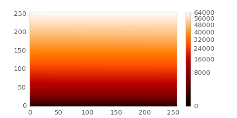
The new Data Visualization package is intended to collect functionality that can be helpful when visualizing data. At the moment, the main functionality is image normalizing (including both scaling and stretching) but this will be expanded in future. Included in the image normalization functionality is the ability to compute interval limits on data, (such as percentile limits), stretching with non-linear functions (such as square root or arcsinh functions), and the ability to use custom stretches in Matplotlib that are correctly reflected in the colorbar:
import numpy as np
import matplotlib.pyplot as plt

from astropy.visualization import SqrtStretch
from astropy.visualization.mpl_normalize import ImageNormalize

# Generate test image
image = np.arange(65536).reshape((256, 256))

# Create normalizer object
norm = ImageNormalize(vmin=0., vmax=65536, stretch=SqrtStretch())

fig = plt.figure(figsize=(6,3))
ax = fig.add_subplot(1,1,1)
im = ax.imshow(image, norm=norm, origin='lower', aspect='auto')
fig.colorbar(im)
(Source code, png, hires.png, pdf)
New analytic functions subpackage
This subpackage provides analytic functions that are commonly used in
astronomy. These already understand Quantity, i.e., they can
handle units of input and output parameters. For instance, to calculate the
blackbody flux for 10000K at 6000 Angstrom:
>>> from astropy import units as u
>>> from astropy.analytic_functions import blackbody_lambda, blackbody_nu
>>> blackbody_lambda(6000 * u.AA, 10000 * u.K)
<Quantity 15315791.836941158 erg / (Angstrom cm2 s sr)>
>>> blackbody_nu(6000 * u.AA, 10000 * u.K)
<Quantity 0.00018391673686797075 erg / (cm2 Hz s sr)
See Analytic Functions (astropy.analytic_functions) for more details.
In future versions of Astropy, the functions in this module might also be
accessible as Model classes.
New ASCII features
Fast readers/writers for ASCII files
The astropy.io.ascii module now includes a significantly faster Cython/C engine
for reading and writing ASCII files. This is available for the following
formats: basic, commented_header, csv, no_header, rdb, and
tab. On average the new engine is about 4 to 5 times faster than the
corresponding pure-Python implementation, and is often comparable to the speed
of the pandas ASCII file
interface (read_csv and
to_csv). The
fast reader has parallel processing option that allows harnessing multiple
cores for input parsing to achieve even greater speed gains.
By default, read() and write()
will attempt to use the fast C engine when dealing with compatible formats.
Certain features of the full read / write interface are not available in the
fast version, in which case the pure-Python version will automatically be used.
For full details including extensive performance testing, see Fast ASCII I/O.
Enhanced CSV format
One of the problems when storing a table in an ASCII format is preserving table meta-data such as comments, keywords and column data types, units, and descriptions. Using the newly defined Enhanced Character Separated Values format it is now possible to write a table to an ASCII-format file and read it back with no loss of information. The ECSV format has been designed to be both human-readable and compatible with most simple CSV readers.
In the example below we show writing a table that has float32 and bool
types. This illustrates the simple look of the format which has a few header
lines (starting with #) in YAML format and then
the data values in CSV format.
>>> t = Table()
>>> t['x'] = Column([1.0, 2.0], unit='m', dtype='float32')
>>> t['y'] = Column([False, True], dtype='bool')

>>> from astropy.extern.six.moves import StringIO
>>> fh = StringIO()
>>> t.write(fh, format='ascii.ecsv')
>>> table_string = fh.getvalue()
>>> print(table_string)
# %ECSV 0.9
# ---
# columns:
# - {name: x, unit: m, type: float32}
# - {name: y, type: bool}
x y
1.0 False
2.0 True
Without the header this table would get read back with different types
(float64 and string respectively) and no unit values. Instead with
the automatically-detected ECSV we get:
>>> Table.read(table_string, format='ascii')
<Table masked=False length=2>
   x      y
   m
float32  bool
------- -----
    1.0 False
    2.0  True
Note that using the ECSV reader requires the PyYAML package to be installed.
New modeling features
New subclasses of Model are now a bit easier to define,
requiring less boilerplate code in general. Now all that is necessary to
define a new model class is an evaluate method that
computes the model. Optionally one can define fittable parameters, a fit_deriv, and/or
an inverse. The new, improved
custom_model decorator reduces the boilerplate needed for
many models even more. See Defining New Model Classes for more details.
Array broadcasting has also been improved, enabling a broader range of possibilities for the values of model parameters and inputs. Support has also been improved for Model Sets (previously referred to as parameter sets) which can be thought of like an array of models of the same class, each with different sets of parameters, which can be fitted simultaneously either to the same data, or to different data sets per model. See Instantiating and Evaluating Models for more details.
It is now possible to create compound models by combining existing models
using the standard arithmetic operators such as + and *, as well as
functional composition using the | operator. This provides a powerful
and flexible new way to create more complex models without having to define
any special classes or functions. For example:
>>> from astropy.modeling.models import Gaussian1D
>>> gaussian1 = Gaussian1D(1, 0, 0.2)
>>> gaussian2 = Gaussian1D(2.5, 0.5, 0.1)
>>> sum_of_gaussians = gaussian1 + gaussian2
The resulting model works like any other model, and also works with the fitting framework. See the introduction to compound models and full compound models documentation for more examples.
New Table features
Refactor of table infrastructure
The underlying data container for the Astropy Table object has been changed
in Astropy v1.0. Previously, tables were stored internally as a Numpy structured
array object, with column access being a memory view of the corresponding Numpy
array field. Starting with this release the fundamental data container is an
ordered dictionary of individual column objects and each Column object is the
sole owner of its data.
The biggest impact to users is that operations such as adding or removing table columns is now significantly faster because there is no structured array to rebuild each time.
For details please see Table implementation change in 1.0.
Support for ‘mixin’ columns
Version v1.0 of Astropy introduces a new concept of the “Mixin
Column” in tables which allows integration of appropriate non-Column based
class objects within a Table object. These mixin column objects are not
converted in any way but are used natively.
The available built-in mixin column classes are Quantity, SkyCoord, and
Time. User classes for array-like objects that support the
Mixin protocol can also be used in tables as mixin columns.
Warning
While the Astropy developers are excited about this new capability and intend to improve it, the interface for using mixin columns is not stable at this point and it is not recommended for use in production code.
As an example we can create a table and add a time column:
>>> from astropy.table import Table
>>> from astropy.time import Time
>>> t = Table()
>>> t['index'] = [1, 2]
>>> t['time'] = Time(['2001-01-02T12:34:56', '2001-02-03T00:01:02'])
>>> print(t)
index           time
----- -----------------------
    1 2001-01-02T12:34:56.000
    2 2001-02-03T00:01:02.000
The important point here is that the time column is a bona fide Time object:
>>> t['time']
<Time object: scale='utc' format='isot' value=['2001-01-02T12:34:56.000' '2001-02-03T00:01:02.000']>
>>> t['time'].mjd
array([ 51911.52425926,  51943.00071759])
For all the details, including a new QTable class, please see Mixin columns.
Integration with WCSAxes
The WCS class can now be used as a Matplotlib projection to make plots of images with WCS
coordinates overlaid, making use of the WCSAxes affiliated package behind the scenes. More
information on using this functionality can be found in the WCSAxes documentation.
Deprecation and backward-incompatible changes
Astropy is now no longer supported on Python 3.1 and 3.2. Python 3.x users should use Python 3.3 or 3.4. In addition, support for Numpy 1.5 has been dropped, and users should make sure they are using Numpy 1.6 or later.
Full change log
To see a detailed list of all changes in version v1.0, including changes in API, please see the Full Changelog.