Data Tables (`astropy.table`)¶

Introduction¶

astropy.table provides functionality for storing and manipulating heterogeneous tables of data in a way that is familiar to numpy users. A few notable capabilities of this package are:

Initialize a table from a wide variety of input data structures and types.
Modify a table by adding or removing columns, changing column names, or adding new rows of data.
Handle tables containing missing values.
Include table and column metadata as flexible data structures.
Specify a description, units and output formatting for columns.
Interactively scroll through long tables similar to using more.
Create a new table by selecting rows or columns from a table.
Perform Table operations like database joins, concatenation, and binning.
Maintain a table index for fast retrieval of table items or ranges.
Manipulate multidimensional columns.
Handle non-native (mixin) column types within table.
Methods for Reading and writing Table objects to files.
Hooks for Subclassing Table and its component classes.

Currently astropy.table is used when reading an ASCII table using astropy.io.ascii. Future releases of AstroPy are expected to use the Table class for other subpackages such as astropy.io.votable and astropy.io.fits .

Note

Starting with version 1.0 of astropy the internal implementation of the Table class changed so that it no longer uses numpy structured arrays as the core table data container. Instead the table is stored as a collection of individual column objects. For most users there is NO CHANGE to the interface and behavior of |Table| objects.

The page on Table implementation change in 1.0 provides details about the change. This includes discussion of the table architecture, key differences, and benefits of the change.

Getting Started¶

The basic workflow for creating a table, accessing table elements, and modifying the table is shown below. These examples show a very simple case, while the full astropy.table documentation is available from the Using table section.

First create a simple table with three columns of data named a, b, and c. These columns have integer, float, and string values respectively:

>>> from astropy.table import Table
>>> a = [1, 4, 5]
>>> b = [2.0, 5.0, 8.2]
>>> c = ['x', 'y', 'z']
>>> t = Table([a, b, c], names=('a', 'b', 'c'), meta={'name': 'first table'})

If you have row-oriented input data such as a list of records, use the rows keyword. In this example we also explicitly set the data types for each column:

>>> data_rows = [(1, 2.0, 'x'),
...              (4, 5.0, 'y'),
...              (5, 8.2, 'z')]
>>> t = Table(rows=data_rows, names=('a', 'b', 'c'), meta={'name': 'first table'},
...           dtype=('i4', 'f8', 'S1'))

There are a few ways to examine the table. You can get detailed information about the table values and column definitions as follows:

>>> t  
<Table length=3>
  a      b     c
int32 float64 str1
----- ------- ----
    1     2.0    x
    4     5.0    y
    5     8.2    z

You can also assign a unit to the columns. If any column has a unit assigned, all units would be shown as follows:

>>> t['b'].unit = 's'
>>> t  
<Table length=3>
  a      b       c
         s
int32 float64 str1
----- ------- ----
    1     2.0    x
    4     5.0    y
    5     8.2    z

Finally, you can get summary information about the table as follows:

>>> t.info  
<Table length=3>
name  dtype  unit
---- ------- ----
   a   int32
   b float64    s
   c    str1

A column with a unit works with and can be easily converted to an Quantity object (but see Quantity and QTable for a way to natively use Quantity objects in tables):

>>> t['b'].quantity
<Quantity [ 2. , 5. , 8.2] s>
>>> t['b'].to('min')  
<Quantity [ 0.03333333, 0.08333333, 0.13666667] min>

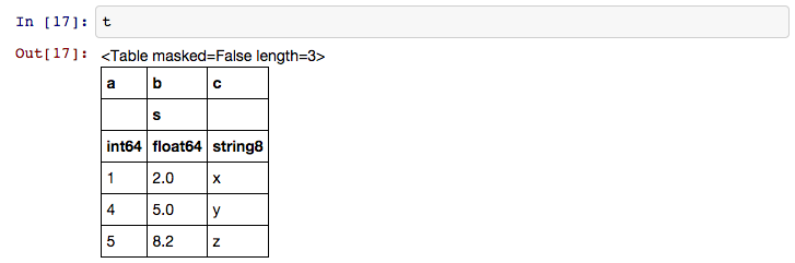
From within the IPython notebook, the table is displayed as a formatted HTML table:

If you print the table (either from the notebook or in a text console session) then a formatted version appears:

>>> print(t)
 a   b   c
     s
--- --- ---
  1 2.0   x
  4 5.0   y
  5 8.2   z

If you do not like the format of a particular column, you can change it:

>>> t['b'].format = '7.3f'
>>> print(t)
 a     b     c
       s
--- ------- ---
  1   2.000   x
  4   5.000   y
  5   8.200   z

For a long table you can scroll up and down through the table one page at time:

>>> t.more()  

You can also display it as an HTML-formatted table in the browser:

>>> t.show_in_browser()  

or as an interactive (searchable & sortable) javascript table:

>>> t.show_in_browser(jsviewer=True)  

Now examine some high-level information about the table:

>>> t.colnames
['a', 'b', 'c']
>>> len(t)
3
>>> t.meta
{'name': 'first table'}

Access the data by column or row using familiar numpy structured array syntax:

>>> t['a']       # Column 'a'
<Column name='a' dtype='int32' length=3>
1
4
5

>>> t['a'][1]    # Row 1 of column 'a'
4

>>> t[1]         # Row object for table row index=1 
<Row index=1>
  a      b     c
         s
int32 float64 str1
----- ------- ----
    4   5.000    y


>>> t[1]['a']    # Column 'a' of row 1
4

You can retrieve a subset of a table by rows (using a slice) or columns (using column names), where the subset is returned as a new table:

>>> print(t[0:2])      # Table object with rows 0 and 1
 a     b     c
       s
--- ------- ---
  1   2.000   x
  4   5.000   y

>>> print(t['a', 'c'])  # Table with cols 'a', 'c'
 a   c
--- ---
  1   x
  4   y
  5   z

Modifying table values in place is flexible and works as one would expect:

>>> t['a'] = [-1, -2, -3]       # Set all column values
>>> t['a'][2] = 30              # Set row 2 of column 'a'
>>> t[1] = (8, 9.0, "W")        # Set all row values
>>> t[1]['b'] = -9              # Set column 'b' of row 1
>>> t[0:2]['b'] = 100.0         # Set column 'b' of rows 0 and 1
>>> print(t)
 a     b     c
       s
--- ------- ---
 -1 100.000   x
  8 100.000   W
 30   8.200   z

Add, remove, and rename columns with the following:

>>> t['d'] = [1, 2, 3]
>>> del t['c']
>>> t.rename_column('a', 'A')
>>> t.colnames
['A', 'b', 'd']

Adding a new row of data to the table is as follows:

>>> t.add_row([-8, -9, 10])
>>> len(t)
4

You can create a table with support for missing values, for example by setting masked=True:

>>> t = Table([a, b, c], names=('a', 'b', 'c'), masked=True, dtype=('i4', 'f8', 'S1'))
>>> t['a'].mask = [True, True, False]
>>> t  
<Table masked=True length=3>
  a      b     c
int32 float64 str1
----- ------- ----
   --     2.0    x
   --     5.0    y
    5     8.2    z

You can include certain object types like Time, SkyCoord or Quantity in your table. These “mixin” columns behave like a hybrid of a regular Column and the native object type (see Mixin columns). For example:

>>> from astropy.time import Time
>>> from astropy.coordinates import SkyCoord
>>> tm = Time(['2000:002', '2002:345'])
>>> sc = SkyCoord([10, 20], [-45, +40], unit='deg')
>>> t = Table([tm, sc], names=['time', 'skycoord'])
>>> t
<Table length=2>
         time          skycoord
                       deg,deg
        object          object
--------------------- ----------
2000:002:00:00:00.000 10.0,-45.0
2002:345:00:00:00.000  20.0,40.0

The QTable class is a variant of Table that allows including a native Quantity in a table instead of converting to a Column object (see Quantity and QTable for details):

>>> from astropy.table import QTable
>>> import astropy.units as u
>>> t = QTable()
>>> t['dist'] = [1, 2] * u.m
>>> t['velocity'] = [3, 4] * u.m / u.s
>>> t
<QTable length=2>
  dist  velocity
   m     m / s
float64 float64
------- --------
    1.0      3.0
    2.0      4.0

Using `table`¶

The details of using astropy.table are provided in the following sections:

I/O with tables¶

Mixin columns¶

Mixin columns

Implementation¶

Reference/API¶

astropy.table Package¶

Functions¶

`hstack`(tables[, join_type, uniq_col_name, ...])	Stack tables along columns (horizontally)
`join`(left, right[, keys, join_type, ...])	Perform a join of the left table with the right table on specified keys.
`unique`(input_table[, keys, silent, keep])	Returns the unique rows of a table.
`vstack`(tables[, join_type, metadata_conflicts])	Stack tables vertically (along rows)

Classes¶

`BST`(data, row_index[, unique])	A basic binary search tree in pure Python, used as an engine for indexing.
`Column`	Define a data column for use in a Table object.
`ColumnGroups`(parent_column[, indices, keys])
`Conf`	Configuration parameters for `astropy.table`.
`FastBST`	alias of `BST`
`FastRBT`	alias of `BST`
`JSViewer`([use_local_files, display_length])	Provides an interactive HTML export of a Table.
`MaskedColumn`	Define a masked data column for use in a Table object.
`NdarrayMixin`	Mixin column class to allow storage of arbitrary numpy ndarrays within a Table.
`QTable`([data, masked, names, dtype, meta, ...])	A class to represent tables of heterogeneous data.
`Row`(table, index)	A class to represent one row of a Table object.
`SortedArray`(data, row_index[, unique])	Implements a sorted array container using a list of numpy arrays.
`Table`([data, masked, names, dtype, meta, ...])	A class to represent tables of heterogeneous data.
`TableColumns`([cols])	OrderedDict subclass for a set of columns.
`TableFormatter`
`TableGroups`(parent_table[, indices, keys])
`TableMergeError`

Data Tables (`astropy.table`)¶

Introduction¶

Getting Started¶

Using `table`¶

Construct table¶

Access table¶

Modify table¶

Table operations¶

Indexing¶

Masking¶

I/O with tables¶

Mixin columns¶

Implementation¶

Reference/API¶

astropy.table Package¶

Functions¶

Classes¶

Class Inheritance Diagram¶

Page Contents

Navigation

Data Tables (astropy.table)¶

Introduction¶

Getting Started¶

Using table¶

Construct table¶

Access table¶

Modify table¶

Table operations¶

Indexing¶

Masking¶

I/O with tables¶

Mixin columns¶

Implementation¶

Reference/API¶

astropy.table Package¶

Functions¶

Classes¶

Class Inheritance Diagram¶

Data Tables (`astropy.table`)¶

Using `table`¶