Image stretching and normalization
The astropy.visualization module provides a framework for transforming values in
images (and more generally any arrays), typically for the purpose of
visualization. Two main types of transformations are provided:
- Normalization to the [0:1] range using lower and upper limits where \(x\) represents the values in the original image:
- Stretching of values in the [0:1] range to the [0:1] range using a linear or non-linear function:
In addition, classes are provided in order to identify lower and upper limits for a dataset based on specific algorithms (such as using percentiles).
Identifying lower and upper limits, as well as re-normalizing, is described in the Intervals and Normalization section, while stretching is described in the Stretching section.
Intervals and Normalization
Several classes are provided for determining intervals and for normalizing values
in this interval to the [0:1] range. One of the simplest examples is the
MinMaxInterval which determines the limits of the
values based on the minimum and maximum values in the array. The class is
instantiated with no arguments:
>>> from astropy.visualization import MinMaxInterval
>>> interval = MinMaxInterval()
and the limits can be determined by calling the
get_limits() method, which takes the
array of values:
>>> interval.get_limits([1, 3, 4, 5, 6])
(1, 6)
The interval instance can also be called like a function to actually
normalize values to the range:
>>> interval([1, 3, 4, 5, 6])
array([ 0. ,  0.4,  0.6,  0.8,  1. ])
Other interval classes include ManualInterval,
PercentileInterval, and
AsymmetricPercentileInterval. For these three,
values in the array can fall outside of the limits given by the interval. A
clip argument is provided to control the behavior of the normalization when
values fall outside the limits:
>>> from astropy.visualization import PercentileInterval
>>> interval = PercentileInterval(50.)
>>> interval.get_limits([1, 3, 4, 5, 6])
(3.0, 5.0)
>>> interval([1, 3, 4, 5, 6])  # default is clip=True
array([ 0. ,  0. ,  0.5,  1. ,  1. ])
>>> interval([1, 3, 4, 5, 6], clip=False)
array([-1. ,  0. ,  0.5,  1. ,  1.5])
Stretching
In addition to classes that can scale values to the [0:1] range, a number of
classes are provide to ‘stretch’ the values using different functions. These
map a [0:1] range onto a transformed [0:1] range. A simple example is the
SqrtStretch class:
>>> from astropy.visualization import SqrtStretch
>>> stretch = SqrtStretch()
>>> stretch([0., 0.25, 0.5, 0.75, 1.])
array([ 0.        ,  0.5       ,  0.70710678,  0.8660254 ,  1.        ])
As for the intervals, values outside the [0:1] range can be treated differently
depending on the clip argument. By default, output values are clipped to
the [0:1] range:
>>> stretch([-1., 0., 0.5, 1., 1.5])
array([ 0.       ,  0.        ,  0.70710678,  1.        ,  1.        ])
but this can be disabled:
>>> stretch([-1., 0., 0.5, 1., 1.5], clip=False)
array([        nan,  0.        ,  0.70710678,  1.        ,  1.22474487])
Note
The stretch functions are similar but not always strictly identical
to those used in e.g. DS9
(although they should have the same behavior). The equations for the
DS9 stretches can be found here
and can be compared to the equations for our stretches provided in
the astropy.visualization API section. The main difference between our
stretches and DS9 is that we have adjusted them so that the [0:1]
range always maps exactly to the [0:1] range.
Combining transformations
Any stretches and intervals can be chained by using the + operator, which
returns a new transformation. For example, to apply normalization based on a
percentile value, followed by a square root stretch, you can do:
>>> transform = SqrtStretch() + PercentileInterval(90.)
>>> transform([1, 3, 4, 5, 6])
array([ 0.        ,  0.60302269,  0.76870611,  0.90453403,  1.        ])
As before, the combined transformation can also accept a clip argument
(which is True by default).
Matplotlib normalization
Matplotlib allows a custom normalization and stretch to be used when showing
data, and requires a Normalize object to be passed
to e.g. imshow(). The astropy.visualization module
provides a class, ImageNormalize, which wraps the
stretch functions from Stretching into an object Matplotlib understands. The
ImageNormalize class takes the limits (which you
can determine from the Intervals and Normalization classes) and the stretch
instance:
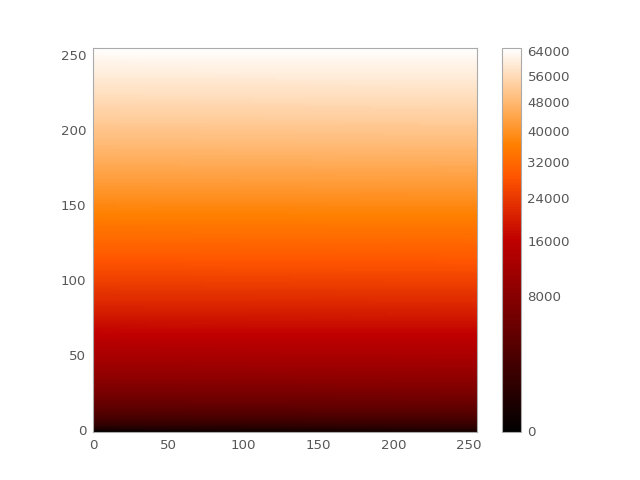
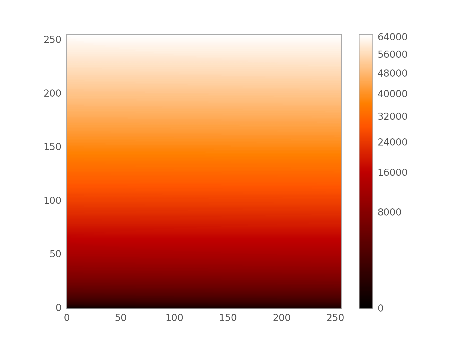
import numpy as np
import matplotlib.pyplot as plt

from astropy.visualization import SqrtStretch
from astropy.visualization.mpl_normalize import ImageNormalize

# Generate test image
image = np.arange(65536).reshape((256, 256))

# Create normalizer object
norm = ImageNormalize(vmin=0., vmax=65536, stretch=SqrtStretch())

# Make the figure
fig = plt.figure()
ax = fig.add_subplot(1, 1, 1)
im = ax.imshow(image, origin='lower', norm=norm)
fig.colorbar(im)
(Source code, png, hires.png, pdf)

As shown above, the colorbar ticks are automatically adjusted.