RunTimePredictor
-
class
astropy.utils.timer.RunTimePredictor(func, *args, **kwargs)[source] [edit on github]¶ Bases:
objectClass to predict run time.
Note
Only predict for single varying numeric input parameter.
Parameters: func : function
Function to time.
args : tuple
Fixed positional argument(s) for the function.
kwargs : dict
Fixed keyword argument(s) for the function.
Examples
>>> from astropy.utils.timer import RunTimePredictor
Set up a predictor for \(10^{x}\):
>>> p = RunTimePredictor(pow, 10)
Give it baseline data to use for prediction and get the function output values:
>>> p.time_func(range(10, 1000, 200))
>>> for input, result in sorted(p.results.items()):
...     print("pow(10, {0})\n{1}".format(input, result))
pow(10, 10)
10000000000
pow(10, 210)
10000000000...
pow(10, 410)
10000000000...
pow(10, 610)
10000000000...
pow(10, 810)
10000000000...
Fit a straight line assuming \(\textnormal{arg}^{1}\) relationship (coefficients are returned):
>>> p.do_fit()
array([1.16777420e-05,  1.00135803e-08])
Predict run time for \(10^{5000}\):
>>> p.predict_time(5000)
6.174564361572262e-05
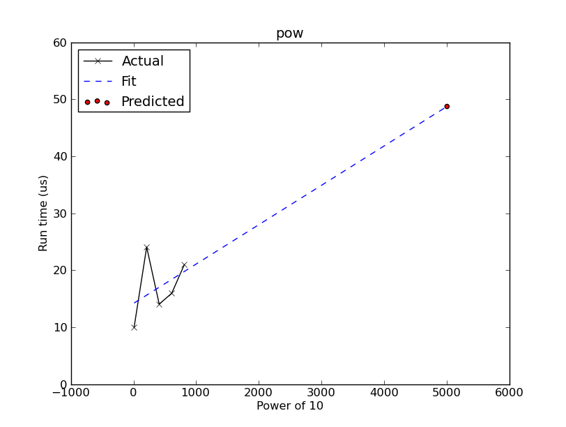
Plot the prediction:
>>> p.plot(xlabeltext='Power of 10')
When the changing argument is not the last, e.g., \(x^{2}\), something like this might work:
>>> p = RunTimePredictor(lambda x: pow(x, 2))
>>> p.time_func([2, 3, 5])
>>> sorted(p.results.items())
[(2, 4), (3, 9), (5, 25)]
Attributes Summary
resultsFunction outputs from time_func.Methods Summary
do_fit([model, fitter, power, min_datapoints])Fit a function to the lists of arguments and their respective run time in the cache. plot([xscale, yscale, xlabeltext, save_as])Plot prediction. predict_time(arg)Predict run time for given argument. time_func(arglist)Time the partial function for a list of single args and store run time in a cache. Attributes Documentation
-
results¶ Function outputs from
time_func.A dictionary mapping input arguments (fixed arguments are not included) to their respective output values.
Methods Documentation
-
do_fit(model=None, fitter=None, power=1, min_datapoints=3)[source] [edit on github]¶ Fit a function to the lists of arguments and their respective run time in the cache.
By default, this does a linear least-square fitting to a straight line on run time w.r.t. argument values raised to the given power, and returns the optimal intercept and slope.
Parameters: model :
astropy.modeling.ModelModel for the expected trend of run time (Y-axis) w.r.t. \(\textnormal{arg}^{\textnormal{power}}\) (X-axis). If
None, will usePolynomial1Dwithdegree=1.fitter :
astropy.modeling.fitting.FitterFitter for the given model to extract optimal coefficient values. If
None, will useLinearLSQFitter.power : int, optional
Power of values to fit.
min_datapoints : int, optional
Minimum number of data points required for fitting. They can be built up with
time_func.Returns: a : array-like
Fitted
FittableModelparameters.Raises: AssertionError
Insufficient data points for fitting.
ModelsError
Invalid model or fitter.
-
plot(xscale=u'linear', yscale=u'linear', xlabeltext=u'args', save_as=u'')[source] [edit on github]¶ Plot prediction.
Note
Uses matplotlib.
Parameters: xscale, yscale : {‘linear’, ‘log’, ‘symlog’}
Scaling for
matplotlib.axes.Axes.xlabeltext : str, optional
Text for X-label.
save_as : str, optional
Save plot as given filename.
Raises: AssertionError
Insufficient data for plotting.
-
predict_time(arg)[source] [edit on github]¶ Predict run time for given argument. If prediction is already cached, cached value is returned.
Parameters: arg : number
Input argument to predict run time for.
Returns: t_est : float
Estimated run time for given argument.
Raises: AssertionError
No fitted data for prediction.
-
time_func(arglist)[source] [edit on github]¶ Time the partial function for a list of single args and store run time in a cache. This forms a baseline for the prediction.
This also stores function outputs in
results.Parameters: arglist : list of numbers
List of input arguments to time.
-